Less can be more in sensor deployment
Despite the ever decreasing prices for Internet-connected devices, sensor deployment doesn’t necessarily become cheaper.
One can still find Arduino-compatible shields in the range of $30+, but in 2014 the ESP8266 chip that was originally marketed as WiFi module for microcontrollers was found to have sufficient horsepower to function as standalone system - for one tenth of the price of a WiFi shield. I can only assume that the price decay is similar when you are an electronics manufacturer and can purchase components in bulk. With the notorious “50 billion connected devices by 2020” we keep hearing about, it is clear that nobody wants to add another 200% to the price of their product just to have it connected.
What might work well in consumer products can be a nightmare in smart city or smart building contexts. Drilling holes into streets, mounting devices on lamp posts or even establishing a basic physical IT infrastructure in an old building doesn’t come cheap. In fact, the price for labour is even likely to increase due to inflation. Everyone in the emerging IoT verticals is trying to pitch the potential savings, but what does it help that the price of an Internet-connected sensor has dropped to cents when its deployment still costs a comparative fortune? Lucky you, because maybe you don’t have to.
Why your data scientist will be grateful for less data
Generally, when you’re trying to address a question with data, the rule is: the more the better. That’s common sense. If you’re allowed a phone call to ask somebody you haven’t seen before five questions about their looks, you’re more likely to recognise them at the airport pickup than when you can only ask them one. But, besides appearing creepy, what would twenty questions do for you? What would you ask? Can you roll your tongue? And what’s the colour of the other eye brow? The first question would probably reveal relatively little information as you don’t have access to this feature when you need it, while the second question is extremely likely to yield redundant information, as most if not all people have same-coloured eye brows.
In every machine learning exercise (be it classification or prediction: the ultimate reason for collecting data in the first place), one of the first steps is feature reduction. Because most calculations are costly and can in the worst case even yield false results, we aim to remove those features that carry only little information to master the task at hand, and a match to two or more different features that are highly correlated (“left eye-brow”, “right eye-brow”) may give us a false sense of knowing already enough. While in our example it’s rather trivial to decide which features should be kept (I’d go for height, hair colour…), a computer needs to produce a correlation matrix first.
In other words, a data scientist’s job is often already half-way done once the data is cleaned and the most predictive features have been identified.
Anecdote: thingslearn originated from a few interesting machine learning problems in molecular biology. We had a really exciting paper on dealing with highly correlated features in genomic data and which of those correlated features are the most predictive and meaningful.
Identifying redundancy: An example
Imagine a company that wants to deploy temperature sensors in a building. What’s a good number of sensors to put in? And at what spacing? This obviously depends on what they want to find out.
Say, it’s a large, open plan office with hot desks, no pun intended, as you can see in a moment: While in principle there is air conditioning that allows spatially defined temperature control, many desks in the office remain unused because people complain about heat. So there’s something to be done.
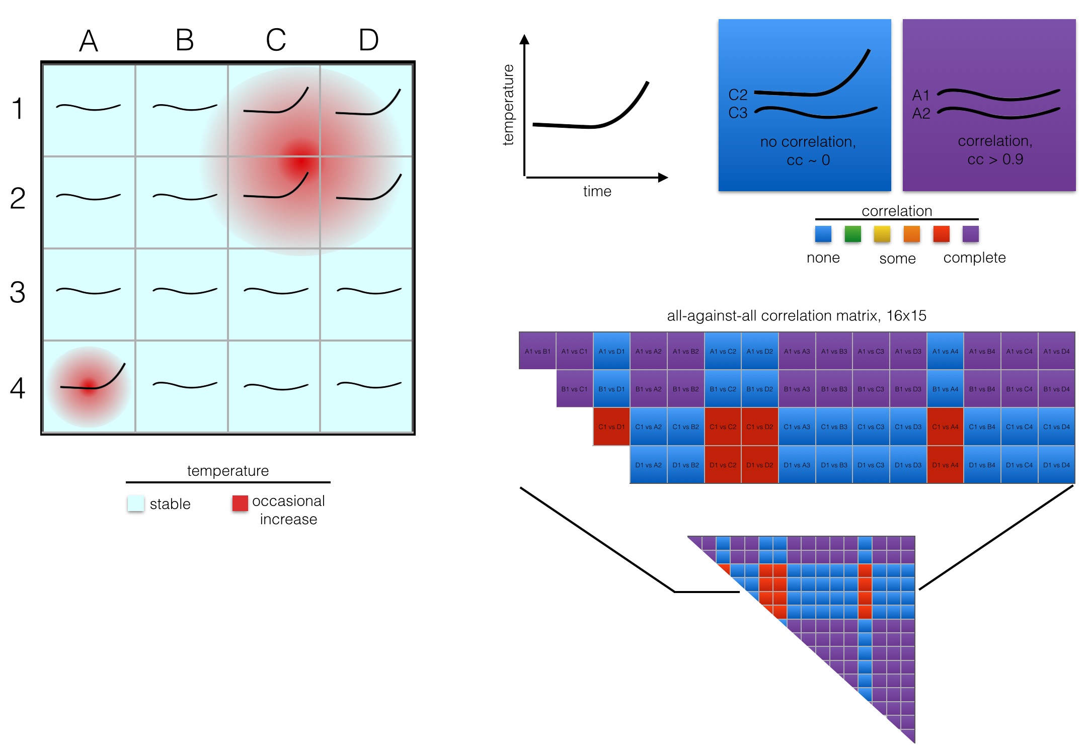
In the example in the figure, when deploying 16 sensors in a 4x4 grid (A1, A2, …, D4), we would find that 5 grid sectors show a profile with increasing temperature over time. Visually, we can immediately recognise that the grid sectors fall into two classes, one with stable temperature and one with instability. When we draw up an all-against-all comparison, we can also infer that computationally.
The temperature profiles are correlated. In other words, whenever any of C1, D1, C2, D2 or A4 go up in temperature, we can infer from our correlation matrix that also the other four in this group are going up, and we should probably intervene. In a machine learning context, we could arbitrarily chose C2, and throw the measurements for C1, D1, D2 and A4 away. That’s what feature reduction does. (In practise it’s not entirely arbitrarily, but for the reason of simplicity we can assume so.)
Practical lesson
What we can learn from above example is the following: Given the prior knowledge of our the temperature profile would suggest that -for the long term- we do only need to deploy a single sensor in this office. We’ve established that most desks are in areas with a stable temperature profile. They won’t need intervention and for this reason we can do without any further measurements. We’ve also established two hot spots with a strong correlative pattern: When the temperature in one hot spot (C1, C2, D1, D2) rises, it’ll also rise in A4. Hence, we could probably manage by just looking at a sensor in one of the hot spot grid sectors.
Now we’ve already invested the money and installed 16 sensors before we have this insight, I hear you say. Well, true, but the lesson here is that a temporary deployment with mobile, leased sensors and analytics on preliminary data can help you save a lot of money. It’s only after this step that you have to decide how many temperature sensors you need to install permanently, with all implications regarding building modification etc.
Other applications
In collaboration with Ethos and OpenSensors we have previously shown the utility of such approach in a smart city context: Parking lots often show correlative patterns, so knowing the occupancy of a few lots allows the prediction of occupancy across a much wider geographical area.
Similar correlative patterns may exist e.g. along the routes of garbage collections. Knowing that, for a particular neighbourhood, the filling level of a few indicative bins allows the driver to skip a few houses can yield significant time savings when accumulated over an entire city.
The above example was obviously full of simplifications. Modern computational methods can take into account any spatio-temporal data, different grid topologies, unevenly distributed sensors and multi-dimensional measurements. If you have any questions and would like to learn more, please do get in touch.